Phylogeographic Temporal Analysis (PTA)

Simulating community-scale co-demographic histories

Questions:

• How do I run PTA simulations?
• What parameters can I change and how do I change them?
• What do the simulations results look like?

Learning objectives:

• Run PTA simulations in the cloud.
• Create, view, and edit the PTA parameters file.
• Understand key model parameters.
• Place prior ranges on model parameters.
• View and interpret simulation outputs.

Table of Contents

• Launch PTA
• Create and edit a new params file
• Running PTA simulations
• Inspecting simulation results

Launch PTA in the cloud

For the purpose of this workshop we are running PTA using Binder, which allows for running github repositories in a free, small and isolated cloud compute instance. This allows us to side-step the (boring) installation process and operate in a homogeneous computing environment.
Click the link below to launch PTA in a new tab.

NOTE: Binder instances are ephemeral!

The down-side of Binder is that the virtual machines they provide are ephemeral, meaning that if you leave it sitting long enough or if you close your tab, everything you have done will be lost. For the purpose of a workshop this is totally fine because we’ll be using toy data and all the steps to reproduce your work will be documented on this page. For the purpose of real work you will not want to use Binder (small amount of resources and inability to save your work), so at the end of the workshop we will provide instructions on how to install PTA and perform analysis on your own computer or HPC system.

That all being said, Binder is still really cool and useful. ;)

After Binder launches you’ll be presented with the JupyterLab interface, which consists of a ‘file browser’ and an ‘app launcher’.

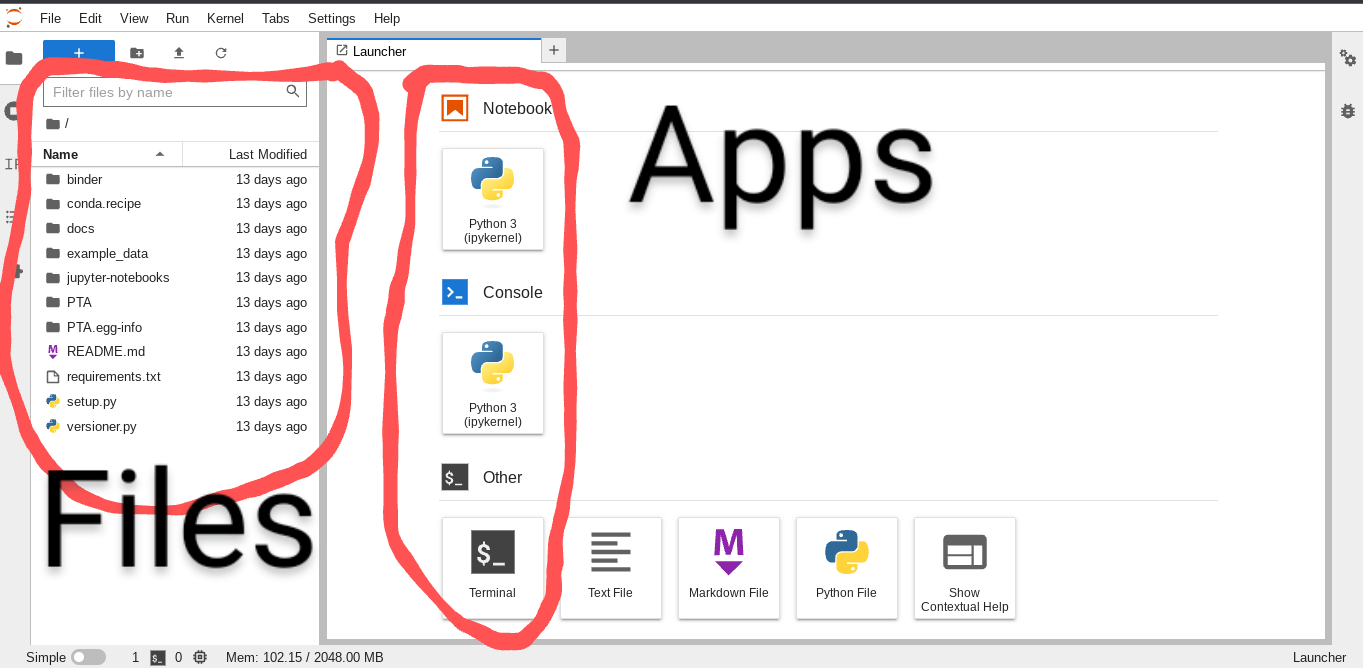
Start by launching a Terminal app, which will bring up a command line interface (CLI). Type PTA and push enter and you’ll see the PTA “Help” message:

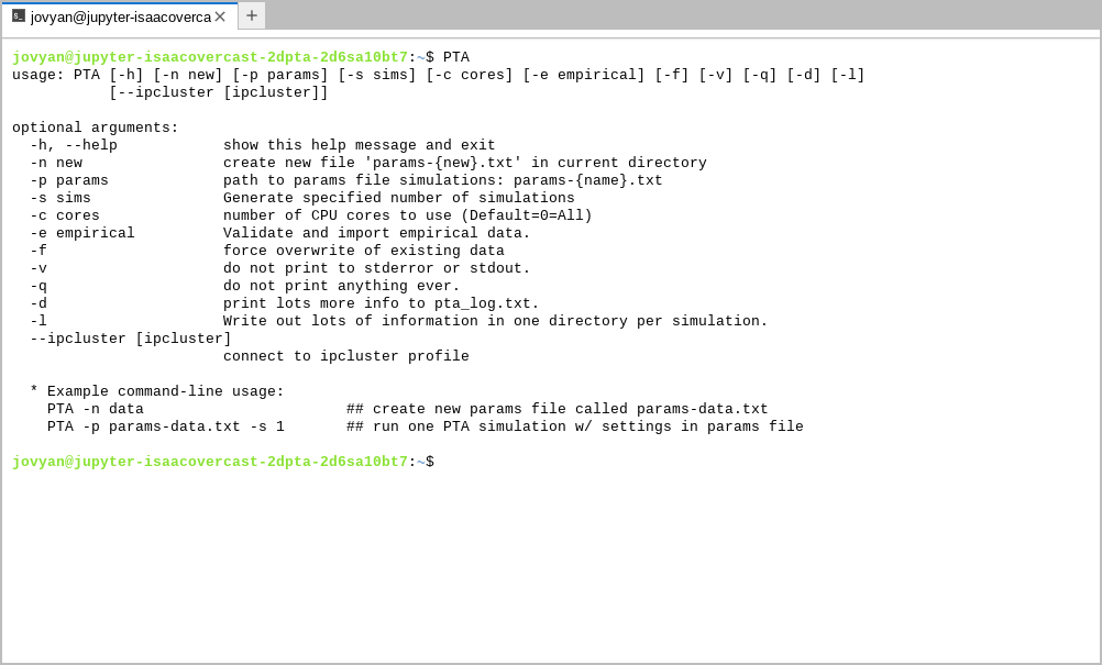
This will show several optional arguments for running PTA, and at the bottom it gives the simplest command-line usage, which involves two steps:

• Creating a ‘params’ file
• Running simulations

So, lets start by creating a params file!

Create and edit a new params file

All PTA simulations are controlled by a ‘params’ file which contains all the settings relevant to the biological processes. The logic of differentiating between parameters in the params file and CLI arguments is to separate the details that are relevant to the biology (params) from the details that are relevant to the execution of the simulations (CLI arguments). You can share a params file with somebody else and they can run simulations on their own computer using CLI arguments that are relevant to the resources available to them (e.g. number of CPU cores) and the simulations they generate will be comparable to those you have generated on your own computer. 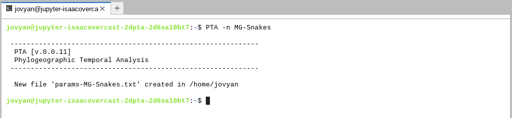The params file encapsulates all the biologically relevant details of the simulations. Let’s make one now by running PTA with the -n flag and specifying a name for our params file (required).

NOTE: On the importance of naming files:

Here we will use Arianna’s Malagasy snake system as inspiration, so we call our params file MG-Snakes. In your own work you should use names for your params files that are meaningful for your system. Also, as usual, spaces are forbidden in params files names.

You can see the newly created file pops up in the file browser on the left side. Double-clicking on the new params-MG-Snakes.txt will pop open this file in a simple text editor interface.

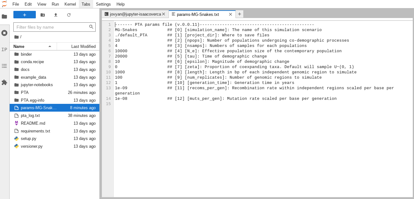
You can see there are (currently) 12 model parameters which describe various aspects of the demographic model and the size and shape of the data to simulate. It can seem a little daunting at first, so lets start with something simple: npops, or the number of ‘populations’ to simulate for our co-demographic analysis. This is simple because typically we will know how many populations there are in our data, so we can just plug in that number for this parameter.

NOTE: By ‘populations’ here what we mean to indicate are the number of independent lineages in the analysis, not specifically ‘populations’ per se. The number of npops could represent species or subspecies or true populations, the taxonomic level isn’t so important as their independence as demographic units within the analysis.

Thinking further in this way we can break the parameters down into two categories: things that we know and things that we want to know. Let’s start with ‘things that we know.’

Things that we know: Parameters that determine the shape and size of the data

The shape and size of the data are things that we know coming into the analysis. By ‘shape and size’ we mean everything having to do with the data that you have in hand in coming to the analysis: number of populations, number of samples per population, length and number of RADSeq loci, and so on. We specify everything that we know about the data to constrain the model to generate simulated data that is as directly comparable to our observed data as possible.

Now let’s edit this file to more closely resemble Arianna’s Malagasy snake data. In the text window change the following values:

21                  ## [2] [npops]: Number of populations undergoing co-demographic processes
6                   ## [3] [nsamps]: Numbers of samples for each populations
100000              ## [4] [N_e]: Effective population size of the contemporary population
150                 ## [8] [length]: Length in bp of each independent genomic region to simulate
0                   ## [11] [recoms_per_gen]: Recombination rate within independent regions scaled per base per generation

Question: Why might we be setting recombs_per_gen to 0 here?

Things that we want to know: Parameters that determine the demographic histories to explore

The demographic history is the unknown process that generated the patterns in the observed data. What we do not know parameters values that determined this process. In order to infer these parameters we must express our uncertainty about their values by placing prior search ranges on them.

For the purpose of this brief tutorial we will focus on only inferring two key model parameters: the proportion of coexpanding taxa [ζ (zeta)] and the timing of co-expansion [τ (tau)]. In practice one might also explore several of the other parameters detailed below, but for computational efficiency we’ll limit ourselves for now. Edit the following lines in the ‘params-MG-Snakes.txt’:

1e5-5e5              ## [5] [tau]: Time of demographic change
0.1                  ## [6] [epsilon]: Magnitude of demographic change
0                    ## [7] [zeta]: Proportion of coexpanding taxa. Default will sample U~(0, 1)

NOTE: In the above 1e5 is a standard scientific notation shortcut to indicate 1*10^5 or 100,000.

NOTE: The meaning of key model parameters

Ne - Effective population size of the contemporary population
τ (tau) - Time of demographic change in years before present
ε (epsilon) - Magnitude of size change backwards in time (ε<1 expansion; ε>1 contraction; ε=1 constant size)
ζ (zeta) - The proportion of co-expanding taxa

When it’s finished, your file should look like this:

------- PTA params file (v.0.0.11)----------------------------------------------
MG-Snakes            ## [0] [simulation_name]: The name of this simulation scenario
./default_PTA        ## [1] [project_dir]: Where to save files
21                   ## [2] [npops]: Number of populations undergoing co-demographic processes
6                    ## [3] [nsamps]: Numbers of samples for each populations
100000               ## [4] [N_e]: Effective population size of the contemporary population
1e5-5e5              ## [5] [tau]: Time of demographic change
0.1                  ## [6] [epsilon]: Magnitude of demographic change
0                    ## [7] [zeta]: Proportion of coexpanding taxa. Default will sample U~(0, 1)
150                  ## [8] [length]: Length in bp of each independent genomic region to simulate
100                  ## [9] [num_replicates]: Number of genomic regions to simulate
1                    ## [10] [generation_time]: Generation time in years
0                    ## [11] [recoms_per_gen]: Recombination rate within independent regions scaled per base per generation
1e-08                ## [12] [muts_per_gen]: Mutation rate scaled per base per generation

After you are done choose File->Save Text to save your changes. Now we are ready to run some simulations!

Challenge: Run 10 simulations

Using the PTA -h help message, see if you can figure out how to run 10 simulations using the params file we just created. Take a few minutes if you need, and try not to peek at the answer below. ;)

Running PTA simulations

If you had luck with the challenge you must have found the -s command-line argument to indicate the number of simulations to run. When running simulations PTA will give a nice progress bar to show you things are running:

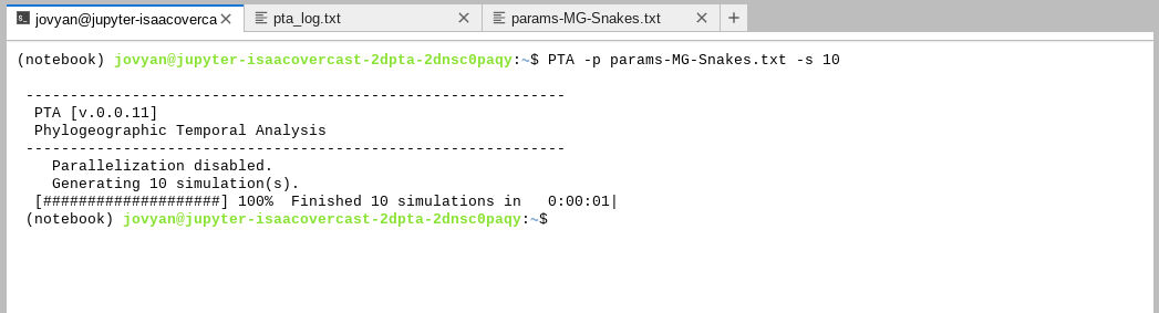
NOTE: Running parallel simulations

You might have noticed in running the simulations that PTA reports Parallelization disabled. This gives you a hint that parallelization is possible! But we don’t need or want to use this on Binder because you only get 1 core anyway, so it wouldn’t improve things to run simulations in parallel. If you run PTA on your on computer or HPC you can use the -c argument to indicate the number of CPU cores to run on, and PTA will automatically split simulations across all these cores. Magic.

OK! So now we ran 10 PTA co-demographic simulations, now what? Well, now first lets take a look at the simulation output to get a better idea of what kind of data the model generates.

Inspecting simulation results

All PTA outputs go in a directory which is specified by the project_dir param in the params file (which by default is default_PTA. The simulated output file shares its name with the params file, so it’s easier to identify which simulations came from which params. Putting that all together, the output file for the simulations we just ran will be: default_PTA/MG-Snakes-SIMOUT.csv

Let us inspect this file using ‘tabview’, a simple csv file viewer which is not natively installed on linux, but which we have included in the binder install for the purpose of making this easier for the workshop. Now open the SIMOUT file by typing: tabview default_PTA/MG-Snakes-SIMOUT.csv

NOTE: Navigate in tabview with the arrow keys and quit by typing q.

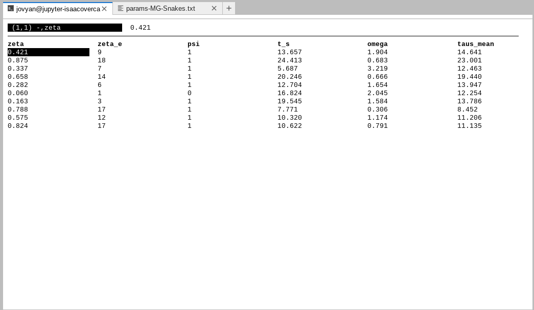
Just like in almost every other case of simulation-based inference, the PTA output file is composed of parameters and data. The parameters come from the values we indicated in the params file, and the data is a summary of the genetic variation generated based on those params.

Spend some time looking at the SIMOUT file. The parameters begin at zeta and end at Ne_s_iqr. Some of these you might recognize (ζ for instance), others are derived from values in the params file (taus_mean is the average time of demographic change for all populations).

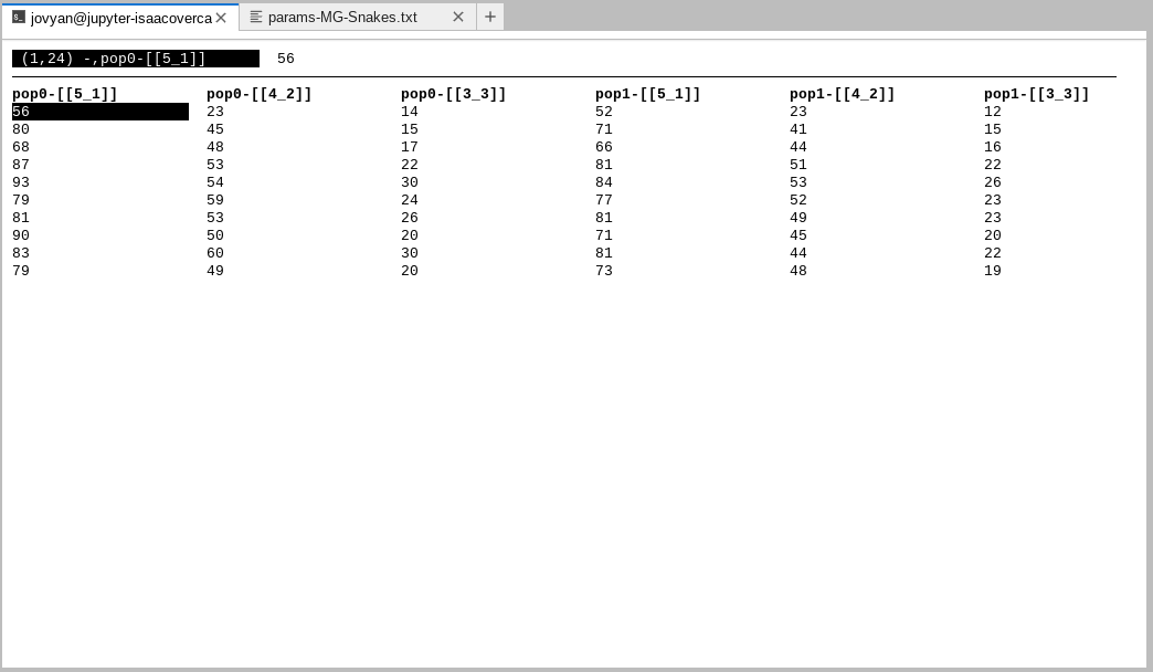
The data begins at pop0-[[5_1]] and continues to the end of the line. All of these somewhat arcane columns record the ‘bins’ of the multi-dimensional site frequency spectrum (mSFS), which is the focal summarization of the genetic data used by PTA.

The goal of simulation based inference is to understand the mapping between the parameters and the data, in other words, how do particular parameter values influence patterns in the data. These days, with very complex and parameter-rich models, we could never hope to do this by eye or even with classical statistical models like linear regression. This is where machine learning comes in, and that will be the focus of our next lesson!

For now let’s take a quick break, and then come back to talk about using PTA simulations for machine learning inference.